Protein-protein binder design with RFdiffusion#
Designing miniprotein binders to IL-7rα with RFdiffusion and ProteinMPNN using the OpenProtein.AI Python client
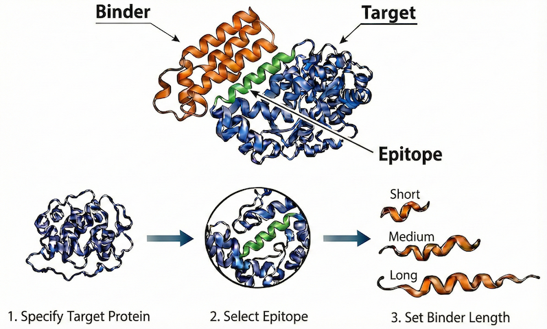
In this tutorial, we’ll demonstrate how to use the OpenProtein.AI Python client to design a protein that binds another protein. We refer to the designed protein as the binder and the protein being bound as the target.
The design process consists of four main steps:
Query Specification: Specify the design problem as a “query”, including
the target protein
the specific epitope that we want to target
the length of binder
Structure Generation: Generate plausible structures for the binder, using RFdiffusion (Watson et al., 2023).
Sequence Design: Design corresponding sequences for each binder structure, using ProteinMPNN (Dauparas et al., 2022).
In Silico Validation: Validate the designed sequences by predicting their structures and computing in silico metrics that are indicative of expression and binding. Filter and select designs for experimental evaluation based on the metrics.
Prerequisites#
To run this tutorial, you’ll need a Python environment containing the following packages:
openprotein_python>=0.10.2molviewspec(for structure visualization)
See the Python client installation instructions for more info.
Additionally, you should have your credentials set up in ~/.openprotein/config.toml to authenticate with the OpenProtein.AI API.
Import necessary packages#
[1]:
from dataclasses import dataclass

import numpy as np
import numpy.typing as npt
import pandas as pd
from scipy.spatial.transform import Rotation

from tqdm import tqdm

import molviewspec as mvs
from molviewspec.nodes import RepresentationTypeT

import openprotein
from openprotein.molecules import Protein, Complex, Structure
Connect to OpenProtein.AI#
[2]:
session = openprotein.connect()
print("✅ Successfully connected to the OpenProtein.AI API!")
✅ Successfully connected to the OpenProtein.AI API!
Step 1: Query Specification#
Specify the protein-protein binder design problem
In this tutorial, we focus on designing a binder for Interleukin-7 receptor alpha (IL-7Rα), a key target in the human immune system. This design problem is adapted from the RFdiffusion study (Watson et al., 2023), which demonstrated the de novo design of high-affinity binders to this target.
In this step, we will create an object, which we refer to as the query, that represents this design problem. The query is defined as a Complex containing two Protein chains: one representing the target and one representing the binder to be designed. We use these classes (Complex and Protein) to specify:
Target: The sequence and structure of the IL-7Rα extracellular domain.
Epitope: The specific residues of IL-7Rα where the binder should bind.
Binder: The desired length of the de novo protein binder.
Step 1.1: Specify the target#
For the IL-7Rα target, we use its structure from RCSB PDB entry 3DI3. We load the PDB entry using Structure.from_pdb_id, which parses the entry into a Structure object. A Structure represents a collection of Complexes, one for each “model” in the PDB entry. In this case, we are only interested in the first and only Complex, which contains our IL-7Rα target. This Complex contains multiple chains; since we’re only interested in our IL-7Rα target, we extract just the
Protein representing the IL-7Rα chain using the Complex.get_protein method:
[3]:
# Load the PDB entry containing the IL-7Rα chain
structure = Structure.from_pdb_id(pdb_id="3DI3")
# Retrieve just the IL-7Rα chain, which is chain B of the first complex
first_complex = structure[0]
target = first_complex.get_protein(chain_id="B")
print("target name:", target.name)
print("target sequence:", target.sequence.decode())
print("target length:", len(target))
target name: 3DI3
target sequence: GSHMESGYAQNGDLEDAELDDYSFSCYSQLEVNGSQHSLTCAFEDPDVNTTNLEFEICGALVEVKCLNFRKLQEIYFIETKKFLLIGKSNICVKVGEKSLTCKKIDLTTIVKPEAPFDLSVVYREGANDFVVTFNTSHLQKKYVKVLMHDVAYRQEKDENKWTHVNLSSTKLTLLQRKLQPAAMYEIKVRSIPDHYFKGFWSEWSPSYYFRTPEINNSSGEMD
target length: 223
Before we continue, we note that although our target protein has 223 residues, the structure at some of these residues is undefined. That is, for some of the residues, the coordinates of their atoms is unknown.
We can track which residues have undefined structure using a structure mask, exposed via Protein.get_structure_mask. The structure mask is a per-residue boolean array indicating whether a residue’s structure is undefined. While this array is useful programmatically, it’s not very informative to inspect directly.
Instead, we visualize the structure mask alongside the sequence using Protein.formatted, which returns a formatted string for pretty printing. In the output below, residues with undefined structure are marked with a caret (^) beneath the corresponding sequence positions.
[4]:
# Visualize the target sequence and its structure mask
print(target.formatted(include=("sequence", "structure_mask")))
0     SEQUENCE       GSHMESGYAQNGDLEDAELDDYSFSCYSQLEVNGSQHSLTCAFEDPDVNTTNLEFEICGA
0     STRUCTURE_MASK ^^^^^^^^^^^^^^^^^^^^

60    SEQUENCE       LVEVKCLNFRKLQEIYFIETKKFLLIGKSNICVKVGEKSLTCKKIDLTTIVKPEAPFDLS
60    STRUCTURE_MASK

120   SEQUENCE       VVYREGANDFVVTFNTSHLQKKYVKVLMHDVAYRQEKDENKWTHVNLSSTKLTLLQRKLQ
120   STRUCTURE_MASK

180   SEQUENCE       PAAMYEIKVRSIPDHYFKGFWSEWSPSYYFRTPEINNSSGEMD
180   STRUCTURE_MASK                                  ^^^^^^^^^^
From the visualization, we can see that the some of the residues at the beginning and end of the target sequence have undefined structure.
To ensure that the design process focuses only on well-defined regions, we should remove these residues with undefined structure from our target object. But before we do that, we’ll define the epitope first below, as it’s slightly easier to identify the binding site before the sequence is modified.
Step 1.2: Specify the epitope#
The epitope is the set of residues in the target that we want our designed binder to bind to. We’ll use the residues at positions 62, 84, and 143 as our epitope; these are the same as the residues used in the RFdiffusion study.
NOTE: When using the API, residues are numbered starting from
1, which follows the canonical mmcif residue id system (label_seq_id), and not the author id system (auth_seq_id).
To specify the epitope, we use the method Protein.set_binding_at. This method is used to specify which residues are the binding residues i.e. the residues that should bind to another protein chain. In this case, that other chain is the binder we’re designing.
[5]:
binding_sites = [62, 84, 143]
target = target.set_binding_at(binding_sites, value="B")
After defining the binding sites, it is helpful to verify their location relative to the protein sequence. We can also use Protein.formatted to visualize the epitope location. In the visualization below, residues marked with B are part of the defined epitope.
[6]:
print(target.formatted(include=("sequence", "binding", "structure_mask")))
0     SEQUENCE       GSHMESGYAQNGDLEDAELDDYSFSCYSQLEVNGSQHSLTCAFEDPDVNTTNLEFEICGA
0     BINDING
0     STRUCTURE_MASK ^^^^^^^^^^^^^^^^^^^^

60    SEQUENCE       LVEVKCLNFRKLQEIYFIETKKFLLIGKSNICVKVGEKSLTCKKIDLTTIVKPEAPFDLS
60    BINDING         B                     B
60    STRUCTURE_MASK

120   SEQUENCE       VVYREGANDFVVTFNTSHLQKKYVKVLMHDVAYRQEKDENKWTHVNLSSTKLTLLQRKLQ
120   BINDING                              B
120   STRUCTURE_MASK

180   SEQUENCE       PAAMYEIKVRSIPDHYFKGFWSEWSPSYYFRTPEINNSSGEMD
180   BINDING
180   STRUCTURE_MASK                                  ^^^^^^^^^^
Remove residues with undefined structure#
Now let’s remove the residues with undefined structure that we discussed earlier. We can do this simply by slicing the target protein using numpy-like slicing syntax, keeping only positions where the structure mask is False.
[7]:
print("target length (old):", len(target))
target = target[~target.get_structure_mask()]
print("target length (new):", len(target))
target length (old): 223
target length (new): 193
Let’s verify by visualizing our target again:
[8]:
print(target.formatted(include=("sequence", "binding", "structure_mask")))
0     SEQUENCE       DYSFSCYSQLEVNGSQHSLTCAFEDPDVNTTNLEFEICGALVEVKCLNFRKLQEIYFIET
0     BINDING                                                 B
0     STRUCTURE_MASK

60    SEQUENCE       KKFLLIGKSNICVKVGEKSLTCKKIDLTTIVKPEAPFDLSVVYREGANDFVVTFNTSHLQ
60    BINDING           B
60    STRUCTURE_MASK

120   SEQUENCE       KKYVKVLMHDVAYRQEKDENKWTHVNLSSTKLTLLQRKLQPAAMYEIKVRSIPDHYFKGF
120   BINDING          B
120   STRUCTURE_MASK

180   SEQUENCE       WSEWSPSYYFRTP
180   BINDING
180   STRUCTURE_MASK
Our visualization shows that regions with undefined structure have now been removed!
Note that by truncating the target, the positions of our binding site have changed. This is why we chose to annotate the binding site first - so that we could simply use the binding site positions aligned to the original target sequence. We can check the positions of the new binding site by looking at the new binding array:
[9]:
# NB: we add one here to get 1-indexed positions
binding_sites = np.where(target.get_binding() == "B")[0] + 1
print("binding site:", binding_sites)
binding site: [ 42 64 123]
Visualize#
It’s always a good idea to visualize the 3D structures of our Proteins to ensure that we’ve created them correctly. First, let’s define a helper function using the molviewspec package to help us create the visualization. It’s not necessary to understand the implementation details.
[10]:
@dataclass(frozen=True)
class ColorSpec:
    chain_id: str
    color: str
    positions: list[int] | None = None
    rep_type: RepresentationTypeT = "cartoon"


def visualize_cif(cif_string: str, colors: list[ColorSpec]):
    builder = mvs.create_builder()
    model = (
        builder.download(url="structure.cif").parse(format="mmcif").model_structure()
    )
    for color_spec in colors:
        component = model.component(
            selector=(
                mvs.ComponentExpression(label_asym_id=color_spec.chain_id)
                if color_spec.positions is None
                else [
                    mvs.ComponentExpression(
                        label_asym_id=color_spec.chain_id, label_seq_id=i
                    )
                    for i in color_spec.positions
                ]
            )
        )
        rep = component.representation(type=color_spec.rep_type)
        rep.color(color=color_spec.color)
    builder.molstar_notebook(
        data={"structure.cif": cif_string},
        width=600,
        height=500,
    )
Before we visualize our target, we rotate it using the method Protein.transform so that the binding site is easy to see in the visualization:
[11]:
# 1. Define the rotation matrix `R`
#    (it's not necessary to understand how we define the rotation matrix `R`)
axis, angle = np.array([-1.0, 1.0, 0.0]), np.radians(45)
R = Rotation.from_rotvec(axis / np.linalg.norm(axis) * angle).as_matrix()
# 2. Apply the rotation
target = target.transform(R=R)
Now, let’s use the helper function, visualize_cif, to visualize our target.
[12]:
visualize_cif(
    cif_string=target.to_string(),
    colors=[
        # color the target chain a light blue
        ColorSpec(chain_id="A", color="#b5e2f5"),
        # color the epitope green, and use the ball_and_stick representation
        ColorSpec(
            chain_id="A",
            color="#6bb50a",
            positions=binding_sites,
            rep_type="ball_and_stick",
        ),
    ],
)
The visualization shows the structure of IL-7Rα, and the epitope comprising three residues spread across three adjacent loop regions, as expected!
Step 1.3: Specify the binder#
For this tutorial, we’ll generate binders of length 80. Since the binder is what we’re designing, its sequence and structure are unknown. To represent this as a Protein object, we simply need to create a Protein of length 80, whose sequence and structure are both undefined! We can do this by simply creating a Protein whose sequence consists of 80 unknown amino acids (unknown is denoted by X); the structure is automatically set to undefined:
[13]:
binder = Protein(sequence="X" * 80)
print("binder length:", len(binder))
binder length: 80
Let’s visualize the binder’s sequence and structure mask to check that they are indeed undefined.
[14]:
print(binder.formatted(include=("sequence", "structure_mask")))
0     SEQUENCE       XXXXXXXXXXXXXXXXXXXXXXXXXXXXXXXXXXXXXXXXXXXXXXXXXXXXXXXXXXXX
0     STRUCTURE_MASK ^^^^^^^^^^^^^^^^^^^^^^^^^^^^^^^^^^^^^^^^^^^^^^^^^^^^^^^^^^^^

60    SEQUENCE       XXXXXXXXXXXXXXXXXXXX
60    STRUCTURE_MASK ^^^^^^^^^^^^^^^^^^^^
As expected, the sequence and structure are both fully undefined.
Finally, now that we have our target and binder, we can combine them into a Complex to form our query! We can do so using the Complex constructor, or more simply, by joining the two Proteins using the & operator like we do below. When combining with &, chain ids are assigned alphabetically, from left to right.
[15]:
query = target & binder
print("Query type", type(query))
print("Chains in query:", list(query.get_chains().keys()))
print("\nVisualize target (Chain A):")
print(query.get_protein(chain_id="A").formatted(include=("sequence", "structure_mask")))
print("\nVisualize binder (Chain B):")
print(query.get_protein(chain_id="B").formatted(include=("sequence", "structure_mask")))
Query type <class 'openprotein.molecules.complex.Complex'>
Chains in query: ['A', 'B']

Visualize target (Chain A):
0     SEQUENCE       DYSFSCYSQLEVNGSQHSLTCAFEDPDVNTTNLEFEICGALVEVKCLNFRKLQEIYFIET
0     STRUCTURE_MASK

60    SEQUENCE       KKFLLIGKSNICVKVGEKSLTCKKIDLTTIVKPEAPFDLSVVYREGANDFVVTFNTSHLQ
60    STRUCTURE_MASK

120   SEQUENCE       KKYVKVLMHDVAYRQEKDENKWTHVNLSSTKLTLLQRKLQPAAMYEIKVRSIPDHYFKGF
120   STRUCTURE_MASK

180   SEQUENCE       WSEWSPSYYFRTP
180   STRUCTURE_MASK

Visualize binder (Chain B):
0     SEQUENCE       XXXXXXXXXXXXXXXXXXXXXXXXXXXXXXXXXXXXXXXXXXXXXXXXXXXXXXXXXXXX
0     STRUCTURE_MASK ^^^^^^^^^^^^^^^^^^^^^^^^^^^^^^^^^^^^^^^^^^^^^^^^^^^^^^^^^^^^

60    SEQUENCE       XXXXXXXXXXXXXXXXXXXX
60    STRUCTURE_MASK ^^^^^^^^^^^^^^^^^^^^
We can now use our query to generate binder designs!
Step 2: Structure Generation#
Generate plausible structures for the binder
In this step, we sample plausible 3D backbones for the binder that geometrically complement the target.
Generate structures with RFdiffusion#
In this tutorial, we use RFdiffusion, a popular structure generation model, to generate the structures. To generate the structures using RFdiffusion, we use the function session.models.rfdiffusion.generate, passing in (1) our query, (2) desired number of structures (N_STRUCTURES=100), and (3) any additional arguments to control the RFdiffusion algorithm.
Below, we run the RFdiffusion job and wait for it to finish; this generally takes about 45 minutes.
[ ]:
N_STRUCTURES = 100

# 1. Create the job
rfdiffusion_job = session.models.rfdiffusion.generate(
    query=query,
    N=N_STRUCTURES,
    # Following Watson et al. (2023), we reduce the noise added during
    # generation, which has been found to help with binder design, albeit at
    # the cost of some diversity.
    **{"denoiser.noise_scale_ca": 0.5, "denoiser.noise_scale_frame": 0.5},
)
print(rfdiffusion_job)

# 2. Wait for the job to finish
_ = rfdiffusion_job.wait_until_done(verbose=True)
job_id='a69af0b5-d318-4bd1-a461-410921a00233' job_type='/models/rfdiffusion' status=<JobStatus.PENDING: 'PENDING'> created_date=datetime.datetime(2026, 1, 17, 4, 17, 1, 686905, tzinfo=TzInfo(0)) start_date=None end_date=None prerequisite_job_id=None progress_message=None progress_counter=0 sequence_length=None
Waiting: 100%|██████████| 100/100 [38:07<00:00, 22.88s/it, status=SUCCESS]
Aside: Easily use different structure generation models by changing a single line of code
The example above uses RFdiffusion for structure generation. To use a different model, all we have to do is change the function we call to that of the corresponding model! For example, if you prefer to use BoltzGen (Stark et al., 2025), the equivalent code is simply:
# BoltzGen-based structure generation
boltzgen_job = session.models.boltzgen.generate(query=query, N=N_STRUCTURES)
Note that we’re calling
session.models.boltzgen.generateinstead ofsession.models.rfdiffusion.generate. The results of this job can be used interchangeably with the results of the RFdiffusion job in the downstream steps of this tutorial.
Next, we retrieve the generated structures as a list of Complex objects.
[17]:
generated_structures: list[Complex] = rfdiffusion_job.get()
assert len(generated_structures) == N_STRUCTURES
print("# of structures generated", len(generated_structures))
# of structures generated 100
Each generated structure is similar to our query, except that the backbone structure of the binder has been filled in by RFdiffusion. Note that the sequence of the binder remains unknown, as we have only generated its backbone structure. Let’s check that this is the case for the first generated structure:
[18]:
first_structure = generated_structures[0]
print("Chains in structure:", sorted(first_structure.get_proteins().keys()))
first_target = first_structure.get_protein(chain_id="A")
first_binder = first_structure.get_protein(chain_id="B")
print("\nVisualize first target (Chain A):")
print(first_target.formatted(include=("sequence", "structure_mask")))
print("\nVisualize first binder (Chain B):")
print(first_binder.formatted(include=("sequence", "structure_mask")))
Chains in structure: ['A', 'B']

Visualize first target (Chain A):
0     SEQUENCE       DYSFSCYSQLEVNGSQHSLTCAFEDPDVNTTNLEFEICGALVEVKCLNFRKLQEIYFIET
0     STRUCTURE_MASK

60    SEQUENCE       KKFLLIGKSNICVKVGEKSLTCKKIDLTTIVKPEAPFDLSVVYREGANDFVVTFNTSHLQ
60    STRUCTURE_MASK

120   SEQUENCE       KKYVKVLMHDVAYRQEKDENKWTHVNLSSTKLTLLQRKLQPAAMYEIKVRSIPDHYFKGF
120   STRUCTURE_MASK

180   SEQUENCE       WSEWSPSYYFRTP
180   STRUCTURE_MASK

Visualize first binder (Chain B):
0     SEQUENCE       XXXXXXXXXXXXXXXXXXXXXXXXXXXXXXXXXXXXXXXXXXXXXXXXXXXXXXXXXXXX
0     STRUCTURE_MASK

60    SEQUENCE       XXXXXXXXXXXXXXXXXXXX
60    STRUCTURE_MASK
As expected, the only thing that has changed from the query is that the binder structure is now fully defined rather than fully undefined, indicating that the binder structure has been generated.
Visualize the generated structures#
Before proceeding, it’s important to visually inspect some of the generated structures to check that they look reasonable and satisfy our query specification.
Visualizing the first structure below, we see that the target-binder complex does indeed satisfy our query specification: the binder is positioned close to the target epitope we specified, and has the right length.
[19]:
visualize_cif(
    generated_structures[0].to_string(),
    colors=[
        ColorSpec(chain_id="A", color="#b5e2f5"),  # target in blue
        ColorSpec(chain_id="B", color="#f4c30b"),  # binder in orange
        ColorSpec(
            chain_id="A",
            color="#6bb50a",  # epitope in green
            positions=binding_sites,
            rep_type="ball_and_stick",
        ),
    ],
)
Looking at another structure below, we see that it also satisfies our query specification. It has a different fold from the first structure, indicating that there is also diversity in the generated binder backbones. Diversity in generated structures is critical for maximizing success, as it increases the effective number of independent hypotheses explored.
[20]:
visualize_cif(
    generated_structures[26].to_string(),
    colors=[
        ColorSpec(chain_id="A", color="#b5e2f5"),  # target in blue
        ColorSpec(chain_id="B", color="#f4c30b"),  # binder in orange
        ColorSpec(
            chain_id="A",
            color="#6bb50a",  # epitope in green
            positions=binding_sites,
            rep_type="ball_and_stick",
        ),
    ],
)
Step 3: Sequence Design#
Design sequences for the binder
In this step, we design sequences for each binder backbone structure using an inverse folding model. We’ll design multiple sequences per structure to increase the chance of designing a sequence that folds into the desired structure.
Design sequences with ProteinMPNN#
In this tutorial, we use ProteinMPNN to design the binder sequences. To generate sequences using ProteinMPNN, we use the function session.models.proteinmpnn.generate, passing in (1) the structure generated by RFdiffusion, (2) the desired number of sequences per structure (N_SEQS_PER_STRUCTURE=10), and (3) any additional arguments to control the ProteinMPNN algorithm.
Below, we run a ProteinMPNN job for every generated structure and wait for the jobs to finish; this generally takes about 15 minutes.
[21]:
N_SEQS_PER_STRUCTURE = 10

# 1. Create the jobs
proteinmpnn_jobs = []
for generated_structure in tqdm(
    generated_structures, mininterval=1.0, desc="Creating jobs"
):
    # 1a. Create a copy of the generated structure with the sequence and side chain
    #     structure of the binder masked.
    #     - It's not actually necessary to do this for this tutorial, as RFdiffusion
    #       already generates binders with the sequence and side chain structure masked.
    #     - However, other structure generation models such as BoltzGen may behave
    #       differently, so doing this ensures that the code is compatbible with
    #       different models.
    generated_structure = generated_structure.copy()
    _ = (
        generated_structure.get_protein(chain_id="B")
        # NB: this mutates the `generated_structure` object
        .mask_sequence()
        .mask_structure(side_chain_only=True)
    )
    # 1b. Create the ProteinMPNN job and store the job
    proteinmpnn_job = session.models.proteinmpnn.generate(
        query=generated_structure,
        num_samples=N_SEQS_PER_STRUCTURE,
        seed=42,  # for reproducibility
    )
    proteinmpnn_jobs.append(proteinmpnn_job)

# 2. Wait for the jobs to finish
for proteinmpnn_job in tqdm(proteinmpnn_jobs, mininterval=1.0, desc="Waiting for jobs"):
    _ = proteinmpnn_job.wait_until_done()
    assert proteinmpnn_job.status == "SUCCESS"
Creating jobs: 100%|██████████| 100/100 [00:31<00:00,  3.20it/s]
Waiting for jobs: 100%|██████████| 100/100 [08:34<00:00,  5.14s/it]
Each ProteinMPNN job returns the designed sequences for the corresponding structure. The designed sequence includes the sequence of both the target and the binder in a colon separated string, ordered by chain id i.e. <target_sequence>:<binder_sequence>.
The sequences of the target returned by ProteinMPNN should always be same as the sequence of the original target as we do not want to redesign the target. On the other hand, the designed sequences of the binders should be novel sequences rather than fully masked sequences of all X.
Let’s retrieve the results of the first ProteinMPNN job to verify that this is the case.
[22]:
first_proteinmpnn_results = proteinmpnn_jobs[0].get()
# inspect first sequence
first_design_seq = first_proteinmpnn_results[0].sequence
first_target_seq, first_binder_seq = first_design_seq.split(":")
assert first_target_seq == target.sequence.decode(), "should match original target"
print("first target sequence", first_target_seq)
print("first binder sequence", first_binder_seq)
# inspect second sequence
second_design_seq = first_proteinmpnn_results[1].sequence
second_target_seq, second_binder_seq = second_design_seq.split(":")
assert second_target_seq == target.sequence.decode(), "should match original target"
print("second target sequence", second_target_seq)
print("second binder sequence", second_binder_seq)
first target sequence DYSFSCYSQLEVNGSQHSLTCAFEDPDVNTTNLEFEICGALVEVKCLNFRKLQEIYFIETKKFLLIGKSNICVKVGEKSLTCKKIDLTTIVKPEAPFDLSVVYREGANDFVVTFNTSHLQKKYVKVLMHDVAYRQEKDENKWTHVNLSSTKLTLLQRKLQPAAMYEIKVRSIPDHYFKGFWSEWSPSYYFRTP
first binder sequence SEKKKEEEKKKNEKFCEETEKESKEEALTEYVEKVKKMYEIEKKYYEEKEKKGEATEEDKKKVEELKKLAEEAEKIKKEK
second target sequence DYSFSCYSQLEVNGSQHSLTCAFEDPDVNTTNLEFEICGALVEVKCLNFRKLQEIYFIETKKFLLIGKSNICVKVGEKSLTCKKIDLTTIVKPEAPFDLSVVYREGANDFVVTFNTSHLQKKYVKVLMHDVAYRQEKDENKWTHVNLSSTKLTLLQRKLQPAAMYEIKVRSIPDHYFKGFWSEWSPSYYFRTP
second binder sequence SLLKKLLEKLKNEKECDETEKESKEEALTKYVEKVEKMYEIKKKEYEEKKKKGEATEEDKKEVEKLKELAEKAKKIKEEK
Each designed sequence is also associated with a score, which indicates the likelihood of the sequence. This score is sometimes used in the in silico validation step, although we do not use it in this tutorial.
[23]:
first_design_score = first_proteinmpnn_results[0].score.item()
second_design_score = first_proteinmpnn_results[1].score.item()
print("first design score", first_design_score)
print("second design score", second_design_score)
first design score 1.1393
second design score 1.1223
Let’s collect all of the designed sequences and scores into a dataframe for further analysis.
[24]:
records = []
for i, proteinmpnn_job in enumerate(tqdm(proteinmpnn_jobs, mininterval=1.0)):
    for j, proteinmpnn_result in enumerate(proteinmpnn_job.get()):
        _, designed_binder_sequence = proteinmpnn_result.sequence.split(":")
        records.append(
            {
                "design_idx": i * N_SEQS_PER_STRUCTURE + j,
                "structure_idx": i,
                "sequence_idx": j,
                "score": proteinmpnn_result.score.item(),
                "sequence": designed_binder_sequence,
            }
        )
df = pd.DataFrame.from_records(records).set_index(["structure_idx", "sequence_idx"])
df.head()
100%|██████████| 100/100 [00:11<00:00, 8.36it/s]
[24]:
| design_idx | score | sequence | ||
|---|---|---|---|---|
| structure_idx | sequence_idx | |||
| 0 | 0 | 0 | 1.1393 | SEKKKEEEKKKNEKFCEETEKESKEEALTEYVEKVKKMYEIEKKYY... |
| 1 | 1 | 1.1223 | SLLKKLLEKLKNEKECDETEKESKEEALTKYVEKVEKMYEIKKKEY... | |
| 2 | 2 | 1.1638 | SLLEALKEKLENEKECEETEKESKEEALTKYVEKVEEMYKIEKEDY... | |
| 3 | 3 | 1.2153 | EEEEKRLLKEEEEKKCEEDEKESEEEALTKYVEKVEKKYEIEKAYY... | |
| 4 | 4 | 1.1442 | KEKEKEERRKKREEEREKTEKESEEEALTKYVEKVKEKYKIEEKYL... |
Step 4: In Silico Validation#
Validate, filter, and select designs using structure prediction
In the last step, we validate our designs by predicting the structure of our designed sequences to
filter for sequences that are likely to adopt the desired structure, and
select promising designs for experimental evaluation based on metrics computed from the predicted structures; these metrics are highly correlated with expression and binding across a variety of previously engineered binders.
Predict structures with Boltz-2#
We predict the structures of our designs using Boltz-2 (Passaro et al., 2025).
Typically, to validate in silico binder designs, we predict the target-binder complex structure and check for consistency with the original designed structure and binding interface. Because the structure of the target is known, but the binder structure is not, we usually run structure prediction in single sequence mode for both the binder and target sequences using only the target structure as a template. Single sequence mode means that no multiple sequence alignment is used for the binder. This is important to efficiently screen large numbers of binder designs where homology search is a bottleneck.
Below, we apply this approach to predict the structures of all designed sequences; this generally takes about 50 minutes.
[ ]:
# 1. Create the complexes to fold
complexes_to_fold = []
for i, generated_structure in enumerate(generated_structures):  # for each structure
    for j in range(N_SEQS_PER_STRUCTURE):
        designed_binder_sequence = df.loc[(i, j)]["sequence"]
        # 1a. Create the complex to fold, containing the target sequence and designed
        #     binder sequence
        complex = Complex(
            {"A": Protein(target.sequence), "B": Protein(designed_binder_sequence)}
        )
        # 1b. Set both the target MSA and the binder MSA to single sequence mode
        complex.get_protein(chain_id="A").msa = Protein.single_sequence_mode
        complex.get_protein(chain_id="B").msa = Protein.single_sequence_mode
        # 1c. Set the known target structure as a template for the target only
        complex.get_protein(chain_id="A").templates = [target]
        complexes_to_fold.append(complex)

# 2. Create the job
fold_job = session.fold.boltz_2.fold(complexes_to_fold)
print(fold_job)

# 3. Wait for the job to finish
_ = fold_job.wait_until_done(verbose=True)
num_records=1000 job_id='a22c1803-97e8-4039-b5c7-acd92a61657e' job_type=<JobType.embeddings_fold: '/embeddings/fold'> status=<JobStatus.PENDING: 'PENDING'> created_date=datetime.datetime(2026, 1, 17, 5, 51, 4, 298027, tzinfo=TzInfo(0)) start_date=None end_date=None prerequisite_job_id=None progress_message=None progress_counter=0 sequence_length=None
Waiting: 100%|██████████| 100/100 [44:01<00:00, 26.42s/it, status=SUCCESS]
We retrieve the predicted structures as a list of Complex objects:
[ ]:
predicted_structures: list[Complex] = []
for structure in fold_job.get(verbose=True):
    # each prediction is a Structure object
    assert isinstance(structure, Structure)
    # since we only make one prediction per design, we extract the `Complex` of that one
    # prediction only, and append that to our list of predicted structures
    predicted_structures.append(structure[0])
Retrieving: 100%|██████████| 1000/1000 [00:23<00:00, 43.30it/s]
Let’s visualize the first predicted structure to check that it looks reasonable:
[29]:
visualize_cif(
    predicted_structures[0]
    .copy()
    .transform(
        # apply a rotation to make the binding site clearer
        # (its not necessary to understand how to define the rotation)
        R=(
            Rotation.from_euler("y", 180, degrees=True)
            * Rotation.from_euler("x", 90, degrees=True)
        ).as_matrix()
    )
    .to_string(),
    colors=[
        ColorSpec(chain_id="A", color="#b5e2f5"),  # target in blue
        ColorSpec(chain_id="B", color="#f4c30b"),  # binder in orange
        ColorSpec(
            chain_id="A",
            color="#6bb50a",  # epitope in green
            positions=binding_sites,
            rep_type="ball_and_stick",
        ),
    ],
)
As expected, the predicted structure contains the target, and the binder close to the target chain.
In addition to the predicted structures, we also retrieve the predicted aligned errors (PAEs), which we will use for computing metrics below. The PAE is a structure prediction confidence metric that has been highly effective at identifying successful binders.
[30]:
predicted_paes: list[npt.NDArray[np.floating]] = fold_job.get_pae()
Filter and select designs by metrics#
We compute, filter, and select designs using standard structure prediction metrics and thresholds adapted from the RFdiffusion study (Watson et al., 2023).
Metric |
Description |
Ideal Value |
|---|---|---|
RMSD |
Measures how closely the predicted structure of the entire complex matches the generated structure. |
< 2.5 Å |
iPAE |
Confidence that the binder forms an interface with the target. |
< 10 |
Binder RMSD |
Measures how closely the predicted structure of just the binder matches the generated structure. |
< 1 Å |
Binder pLDDT |
Confidence in the predicted structure of the binder. |
> 80 |
Compute Metrics#
Below, we compute these metrics and collate the metrics and designed sequences into a dataframe for further analysis.
[31]:
records = []  # collect metrics and designed sequences into a list of records
for i, generated_structure in enumerate(tqdm(generated_structures, mininterval=1.0)):
    for j in range(N_SEQS_PER_STRUCTURE):
        predicted_structure = predicted_structures[i * N_SEQS_PER_STRUCTURE + j]
        # compute overall rmsd
        rmsd = predicted_structure.rmsd(generated_structure)
        # compute ipae
        pae = predicted_paes[i * N_SEQS_PER_STRUCTURE + j].squeeze(0)
        ipae0 = np.mean(pae[: len(target), len(target) :])
        ipae1 = np.mean(pae[len(target) :, : len(target)])
        ipae = (ipae0 + ipae1) / 2
        # compute binder metrics
        generated_binder = generated_structure.get_protein(chain_id="B")
        predicted_binder = predicted_structure.get_protein(chain_id="B")
        binder_rmsd = predicted_binder.rmsd(generated_binder)
        binder_plddt = predicted_binder.plddt.mean()
        # get dataframe row containing designed sequence
        row = df.loc[(i, j)]
        # record all relevant data
        records.append(
            {
                "design_idx": row["design_idx"],
                "structure_idx": i,
                "sequence_idx": j,
                "rmsd": rmsd,
                "ipae": ipae,
                "binder_rmsd": binder_rmsd,
                "binder_plddt": binder_plddt,
                "score": row["score"],
                "sequence": row["sequence"],
            }
        )
df = pd.DataFrame.from_records(records).set_index(["structure_idx", "sequence_idx"])
df.head()
100%|██████████| 100/100 [00:00<00:00, 135.58it/s]
[31]:
| design_idx | rmsd | ipae | binder_rmsd | binder_plddt | score | sequence | ||
|---|---|---|---|---|---|---|---|---|
| structure_idx | sequence_idx | |||||||
| 0 | 0 | 0 | 9.260719 | 19.434719 | 9.555878 | 75.917442 | 1.1393 | SEKKKEEEKKKNEKFCEETEKESKEEALTEYVEKVKKMYEIEKKYY... |
| 1 | 1 | 10.299928 | 24.854660 | 8.796905 | 79.105263 | 1.1223 | SLLKKLLEKLKNEKECDETEKESKEEALTKYVEKVEKMYEIKKKEY... | |
| 2 | 2 | 11.313936 | 9.122387 | 9.742312 | 92.411514 | 1.1638 | SLLEALKEKLENEKECEETEKESKEEALTKYVEKVEEMYKIEKEDY... | |
| 3 | 3 | 14.616865 | 21.523405 | 9.792756 | 90.185501 | 1.2153 | EEEEKRLLKEEEEKKCEEDEKESEEEALTKYVEKVEKKYEIEKAYY... | |
| 4 | 4 | 18.907486 | 14.846831 | 8.477175 | 88.929916 | 1.1442 | KEKEKEERRKKREEEREKTEKESEEEALTKYVEKVKEKYKIEEKYL... |
Filter and select designs by metrics#
We start by filtering the designs based on the ideal metric thresholds.
[32]:
df_filtered = df[
    (df["rmsd"] < 2.5)
    & (df["ipae"] < 10)
    & (df["binder_rmsd"] < 1)
    & (df["binder_plddt"] > 80)
]
print("# designs passing filters", len(df_filtered))
print(
    "# unique structures passing filters",
    df_filtered.index.get_level_values("structure_idx").nunique(),
)
# designs passing filters 253
# unique structures passing filters 58
Looks like we have a good number of designs meeting the ideal metric thresholds!
Next, we rank the designs based on iPAE to prioritize designs with high confidence of interaction. We’ll also select just the top design per unique structure, to select for a diverse set of binders.
[46]:
df_selected = (
    # rank by ipae
    df_filtered.reset_index().sort_values(by="ipae")
    # select best sequence per structure
    .groupby("structure_idx", sort=False).first()
    # set dataframe index
    .reset_index().set_index(["structure_idx", "sequence_idx"])
)
df_selected.head(7)
[46]:
| design_idx | rmsd | ipae | binder_rmsd | binder_plddt | score | sequence | ||
|---|---|---|---|---|---|---|---|---|
| structure_idx | sequence_idx | |||||||
| 26 | 3 | 263 | 0.999716 | 3.776477 | 0.642081 | 95.725227 | 0.9233 | SIEELLKKIKEAAEKGDIEKAIEYLEKLAKKLKEKGYEAENAIALA... |
| 69 | 2 | 692 | 1.127977 | 3.945726 | 0.656315 | 96.416939 | 0.9907 | SKVEELKIELIRGYALYLLLEKKGKYKELAEHLKKEIKKLEEELKK... |
| 59 | 9 | 599 | 2.210228 | 3.961442 | 0.537537 | 95.357101 | 0.8976 | EEKKKEAKKLFEKSSELVEKGIETGSAELIEKGKEYAKKGFDIEIE... |
| 88 | 5 | 885 | 1.169592 | 4.049241 | 0.796574 | 93.093887 | 0.9981 | SEKEELLKKKEEELNKLVEELAKLLPPEAAKEYKEAFEESLELLRE... |
| 13 | 6 | 136 | 1.222657 | 4.107286 | 0.677419 | 95.852638 | 0.9842 | MEELKEEIIKWLEELAKKAPEMNEEEAKKAIEEVAKKLIEVGFSEE... |
| 53 | 0 | 530 | 1.986973 | 4.143474 | 0.801762 | 93.240982 | 1.1098 | LTPEQKAELEAKRKALEEKKKEEKKKYEEEKKKVEELYKKDKKKAK... |
| 42 | 8 | 428 | 1.478008 | 4.226676 | 0.961525 | 94.260635 | 1.0996 | EKEEKEESFESAEKKAEELLKDEKTKKLGEAYKEVLKLIKEGEKKK... |
We now have a ranked list of promising binder designs!
Before we send them off for experimental validation, we should visually inspect their stuctures for any anomalies. For example, below we visualize the predicted structure of the top ranked design superimposed onto the corresponding generated structure (light gray) and see that it looks reasonable on visual inspection:
[ ]:
# get predicted and generated structure of top design
design_idx, structure_idx = df_selected.reset_index().iloc[0][
    ["design_idx", "structure_idx"]
]
predicted_structure = predicted_structures[design_idx]
generated_structure = generated_structures[structure_idx]
# superimpose predicted structure on the generated structure
predicted_structure = predicted_structure.copy().superimpose_onto(generated_structure)
# visualize
visualize_cif(
    Complex(
        {
            "A_predicted": predicted_structure.get_protein(chain_id="A"),
            "B_predicted": predicted_structure.get_protein(chain_id="B"),
            "A_generated": generated_structure.get_protein(chain_id="A"),
            "B_generated": generated_structure.get_protein(chain_id="B"),
        }
    ).to_string(),
    colors=[
        ColorSpec(chain_id="A_predicted", color="#b5e2f5"),
        ColorSpec(chain_id="B_predicted", color="#f4c30b"),
        ColorSpec(
            chain_id="A_predicted",
            color="#6bb50a",
            positions=binding_sites,
            rep_type="ball_and_stick",
        ),
        ColorSpec(chain_id="A_generated", color="#F2F0EF"),
        ColorSpec(chain_id="B_generated", color="#F2F0EF"),
    ],
)
However, the sixth design may be undesirable in some cases because it consists of exactly two alpha helices - previous works have found these structures to be less likely to express in solution.
[ ]:
# get predicted and generated structure of top sixth design
design_idx, structure_idx = df_selected.reset_index().iloc[5][
    ["design_idx", "structure_idx"]
]
predicted_structure = predicted_structures[design_idx]
generated_structure = generated_structures[structure_idx]
# superimpose predicted structure on the generated structure
predicted_structure = predicted_structure.copy().superimpose_onto(generated_structure)
# visualize
visualize_cif(
    Complex(
        {
            "A_predicted": predicted_structure.get_protein(chain_id="A"),
            "B_predicted": predicted_structure.get_protein(chain_id="B"),
            "A_generated": generated_structure.get_protein(chain_id="A"),
            "B_generated": generated_structure.get_protein(chain_id="B"),
        }
    ).to_string(),
    colors=[
        ColorSpec(chain_id="A_predicted", color="#b5e2f5"),
        ColorSpec(chain_id="B_predicted", color="#f4c30b"),
        ColorSpec(
            chain_id="A_predicted",
            color="#6bb50a",
            positions=binding_sites,
            rep_type="ball_and_stick",
        ),
        ColorSpec(chain_id="A_generated", color="#F2F0EF"),
        ColorSpec(chain_id="B_generated", color="#F2F0EF"),
    ],
)
After visually confirming the designs and further filtering based on any additional metrics you may have in mind (e.g. metrics relevant to your specific assay), the designs can then be sent off for experimental testing!
Conclusion#
In this tutorial, we’ve demonstrated how to design novel binders for a target of interest. We validated the designs using in-silico metrics and visualized them to ensure their viability. The top-ranked designs from this workflow can be:
Expressed and purified for experimental validation
Tested for binding affinity
Further optimized through additional rounds of design, for example, with OpenProtein.AI’s property regression models.
Read more about our binder design workflows and other de novo design tools here:
or see the detailed API references