Designing libraries of multimeric proteins#
Introduction#
Protein engineers must be able to work with and design multimeric proteins; a holistic understanding of proteins and their subunits is essential to creating customized protein designs. This walkthrough will cover designing multimeric proteins, using antibodies as our example. The design process for monomeric proteins is shown in Lead optimization of monoclonal antibody to meet target product profile.
When designing proteins with quaternary structures, we must account for the impact of mutations on interaction points between subunits. Antibodies are made up of two light chains and two heavy chains held together by disulfide bonds. Because both the light chains and heavy chains are involved in binding to the target molecule, there may be synergistic mutations in both chains that can improve binding which can’t be found when optimizing each chain in isolation. In addition, optimizing the subunits together prevents disruption of interacting residues and loss in stability and function of the protein complexes. For example, changes to key cysteine residues in full length and Fab antibodies can disrupt interchain disulfide bonds that are key to their function.
In this walkthrough, we will:
visualize the structure of a multimeric protein
upload a dataset
perform in silico design of variant libraries for a multimeric protein
We’ll use flexible linkers to train a single model to design multimeric proteins. The linkers will connect the different subunits in silico, creating a super sequence consisting of multiple polypeptide chains, akin to a single-chain variable fragment (scFv). This will allow the model to treat the overall amino acid sequence as a single protein.
What you need before getting started#
Before getting started we generally recommend:
A library size that contains at least 30 variants. If you are using a smaller library, review the cross-validation results of your model. The library should span mutations across all of the subunits, not just one.
Semi-quantitative or quantitative binding data or measurements on properties of interest. Assays to consider are surface plasmon resonance (SPR), biolayer interferometry (BLI) or enzyme-linked immunosorbent assay (ELISA). This data should include replicates to reduce noise contribution from assay.
Libraries should have mutations across more than one site as well as mutations of different types. For example, alanine scanning can be complemented with substitution of other amino acids at specific sites.
A dataset formatted as a CSV file. See Uploading your data for more information.
Multichain sequence input#
We will be using the data from the single-chain variable fragment (scFv) library described in the paper “Machine learning optimization of candidate antibody yields highly diverse sub-nanomolar affinity antibody libraries” (https://doi.org/10.1038/s41467-023-39022-2).
The scFv protein from this study consists of a heavy chain, a flexible linker (GGGGSX3) and a light chain.
Note: Although the sequences in the provided dataset only have mutations on either the heavy or light chain, the assays performed using scFvs had expressed each variant together with its requisite wild-type heavy or light chain.
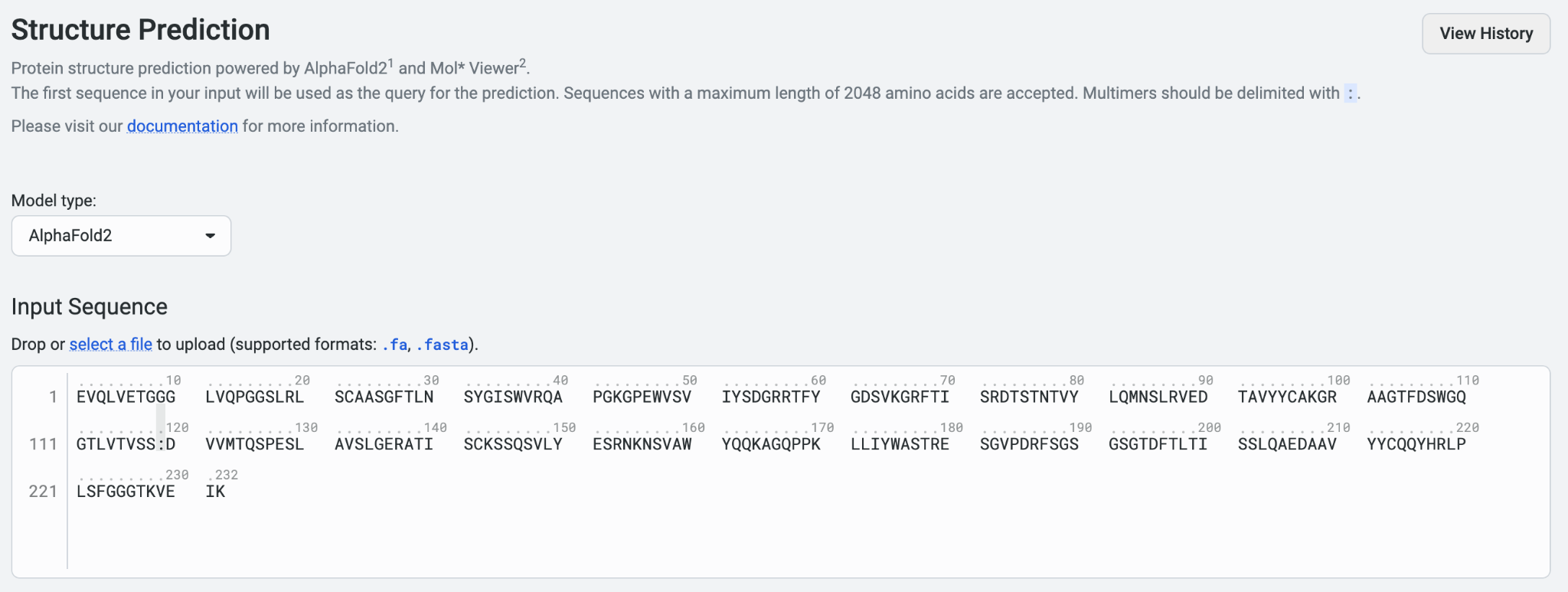
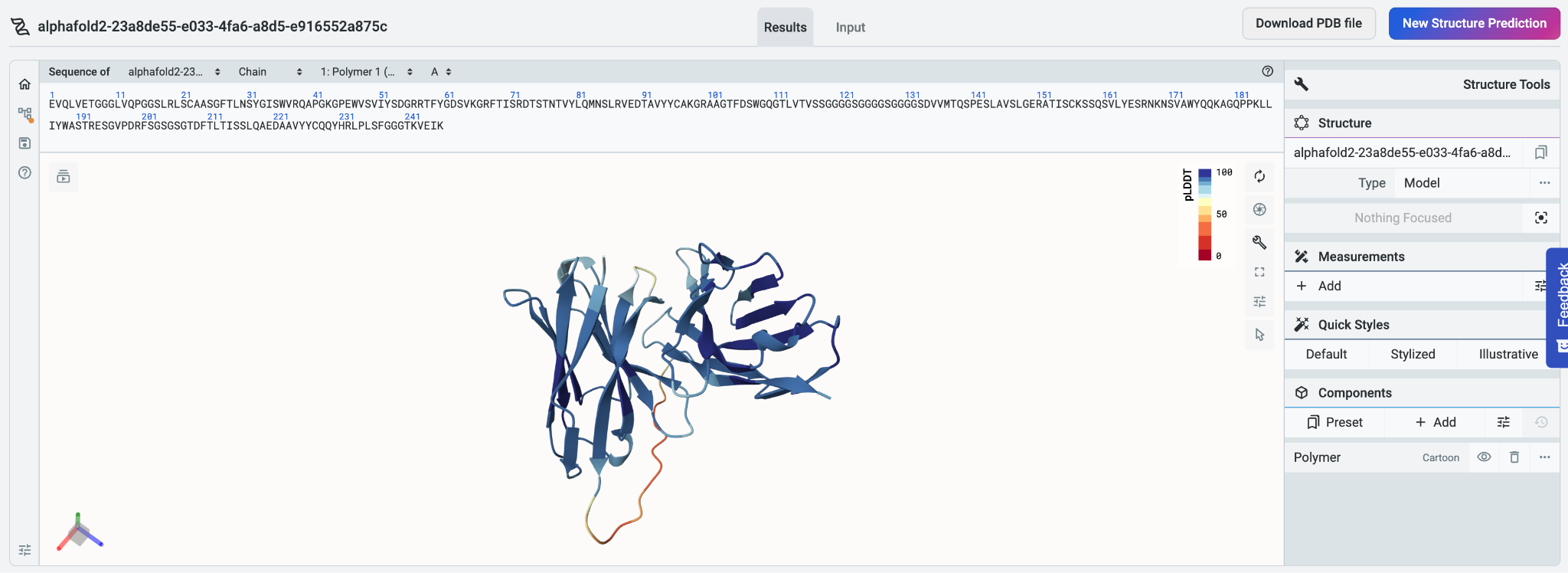
The heavy chain (14H), the flexible linker, and the light chain (14L) components of the wild-type scFv are shown below.
>14H sequence

EVQLVETGGGLVQPGGSLRLSCAASGFTLNSYGISWVRQAPGKGPEWVSVIYSDGRRTFYGDSVKGRFTISRDTSTNTVYLQMNSLRVEDTAVYYCAKGRAAGTFDSWGQGTLVTVSS

>linker sequence

GGGGSGGGGSGGGGS

>14L sequence

DVVMTQSPESLAVSLGERATISCKSSQSVLYESRNKNSVAWYQQKAGQPPKLLIYWASTRESGVPDRFSGSGSGTDFTLTISSLQAEDAAVYYCQQYHRLPLSFGGGTKVEIK
Predicting the structure of the multimeric protein#
Before designing a multimeric protein, it can be useful to examine the positions of the subunits relative to one another. We’ll use the Structure Prediction tool to visualize the structure of our multimeric protein, selecting AlphaFold2 in the tool’s Model type menu.
Note: The AlphaFold2 model is more accurate for multichain analysis.
There are two ways to in silico “chain” together the different subunits in the Input sequence box. The first option is to use a colon (:) between the chains. The inclusion of the colon tells the system that the sequence is made up of subunits. The tool will then add a virtual linker. Alternatively, you can input the full protein sequence consisting of all subunits connected with your flexible linker(s) of choice. We’ll use both methods in our walkthrough, starting with adding a colon to the sequence box between the heavy chain and light chain.
>14H + L sequence
EVQLVETGGGLVQPGGSLRLSCAASGFTLNSYGISWVRQAPGKGPEWVSVIYSDGRRTFYGDSVKGRFTISRDTSTNTVYLQMNSLRVEDTAVYYCAKGRAAGTFDSWGQGTLVTVSS:DVVMTQSPESLAVSLGERATISCKSSQSVLYESRNKNSVAWYQQKAGQPPKLLIYWASTRESGVPDRFSGSGSGTDFTLTISSLQAEDAAVYYCQQYHRLPLSFGGGTKVEIK
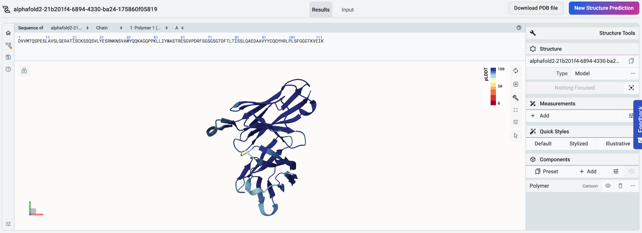
Because we used a colon to split up the chains, Mol* Viewer visualizes the chains as separate polymers instead of treating them as a single polymer. The predicted structures for both chains are shown in the Mol* Viewer implementation on the system, which lets us perform simple manipulations in the Mol* Viewer environment.
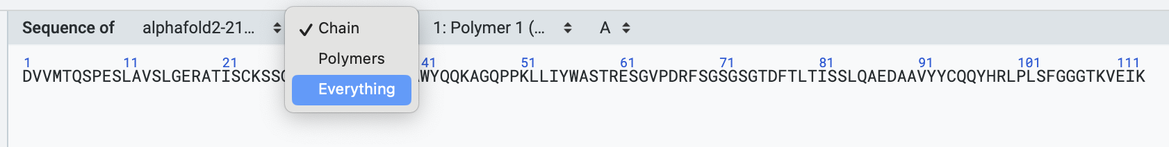
To select residues across both chains using their sequences, we can select Everything in the drop down menu above the sequence to reveal both chains’ sequences for easier manipulation. The structures of all the sequences will be shown regardless of selection.
To measure the distance between the C-terminus of the first subunit to the N-terminus of the second subunit, we first switch tools to the select tool and select the two residues of interest in the sequence space as shown above for Polymer 1: K113 and Polymer 2: E1.
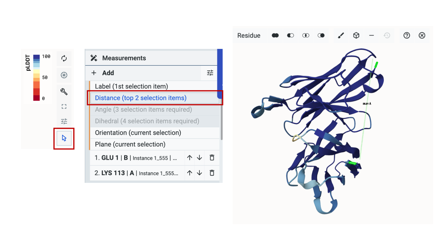
We’ll select +Add, then Distance (top 2 selection items). We can now see that the measured distance between the residues is 35.8 angstroms.
As the axial distance of an amino acid is about 3.5 angstroms, a minimum of 12 amino acids would be needed for a linker. Generally, we’d ensure that proper folding can occur by choosing a longer linker to provide buffer space and flexibility.
For sFvs, the choice of linker is generally GGGGSX3, which has been shown to allow proper folding of both domains. We can chain together subunits in the Input sequence box by adding the flexible linker GGGGSX3 to the amino acid sequence. For other multimeric proteins, it would be useful to test different linkers as needed.
>14H + linker + 14L

EVQLVETGGGLVQPGGSLRLSCAASGFTLNSYGISWVRQAPGKGPEWVSVIYSDGRRTFYGDSVKGRFTISRDTSTNTVYLQMNSLRVEDTAVYYCAKGRAAGTFDSWGQGTLVTVSSGGGGSGGGGSGGGGSDVVMTQSPESLAVSLGERATISCKSSQSVLYESRNKNSVAWYQQKAGQPPKLLIYWASTRESGVPDRFSGSGSGTDFTLTISSLQAEDAAVYYCQQYHRLPLSFGGGTKVEIK
To further analyze our structure, we can select Download PDB file. The resulting file can be used with molecular visualization programs like Chimera X or PyMol.
Our next step is to use OP Models to design a protein variant library.
Using OP Models on multichain proteins#
We’ll start by generating a variant library using the full length scFv data consisting of both the heavy and light chain. We’ll then compare the designed variant library using the multichain input to libraries designed using single chain inputs. The combined data from Li et al., where each variant is paired with the requisite parental sequence and flexible linker, can be downloaded here alongside the single libraries.
Preparing and uploading our data#
We can upload each dataset by selecting Upload dataset and navigating to the CSV file in the file explorer, taking care to upload each file to the same project. The platform will automatically generate the data categories, but it’s important to ensure that the OpenProtein.AI platform has captured the correct names and column types.
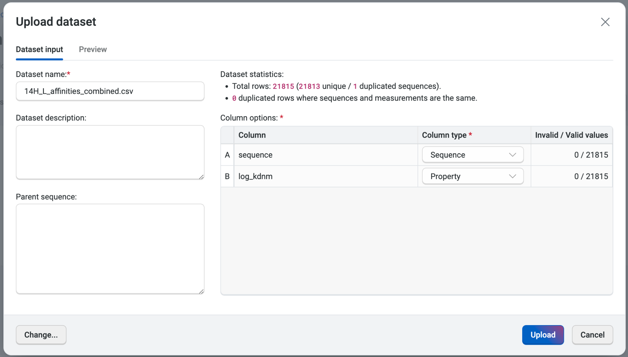
Here, the sequence correctly appears as Sequence and the log_kdnm correctly appears as Property. We’ll also verify that there are no non-numerical values in the dataset, as these are invalid.
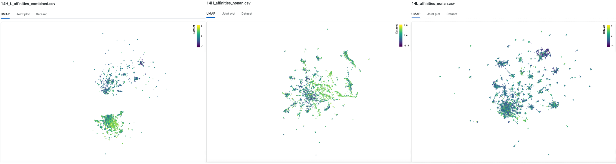
Looking at the multichain library in the UMAP, we can observe that the heavy chain and light chain libraries are fairly distant from each other. This is expected as the heavy chain variants share an identical cognate light chain. Conversely, the light chain variants share an identical cognate heavy chain. By considering both heavy and light chains as a multichain library, we can access a larger protein landscape across the individual clusters and sample mutations that allows us to access a bigger evolutionary landscape.
Training our custom model#
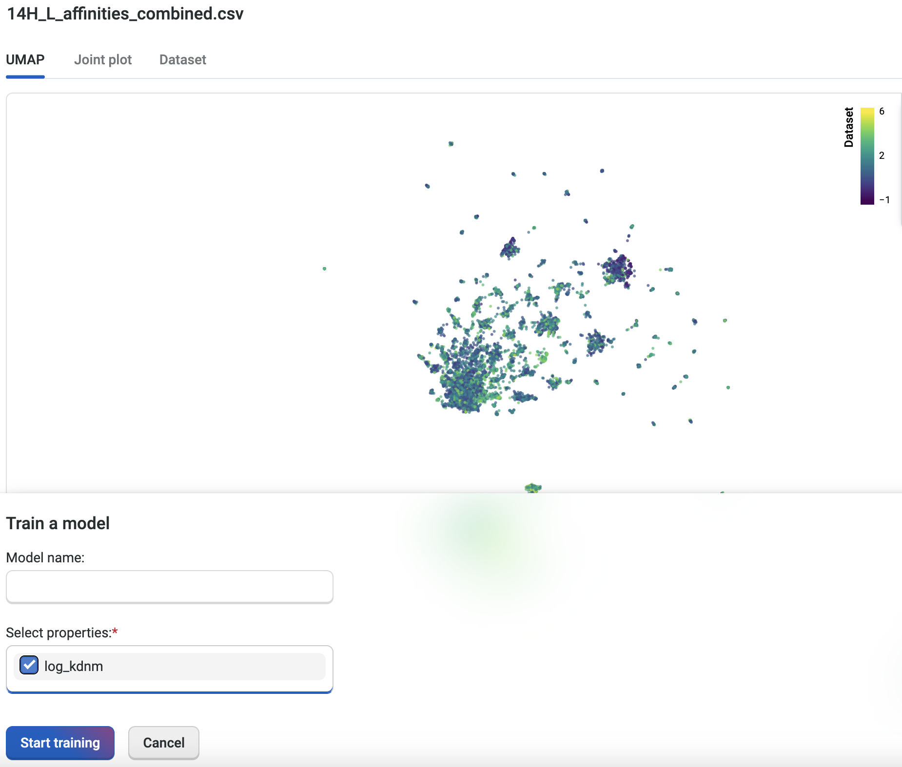
We will now train a custom model for each of our three datasets. The custom model allows us to set specific properties of interest; in this case, we’re using the log Kd measurement to create a model capable of predicting better binders for all three libraries.
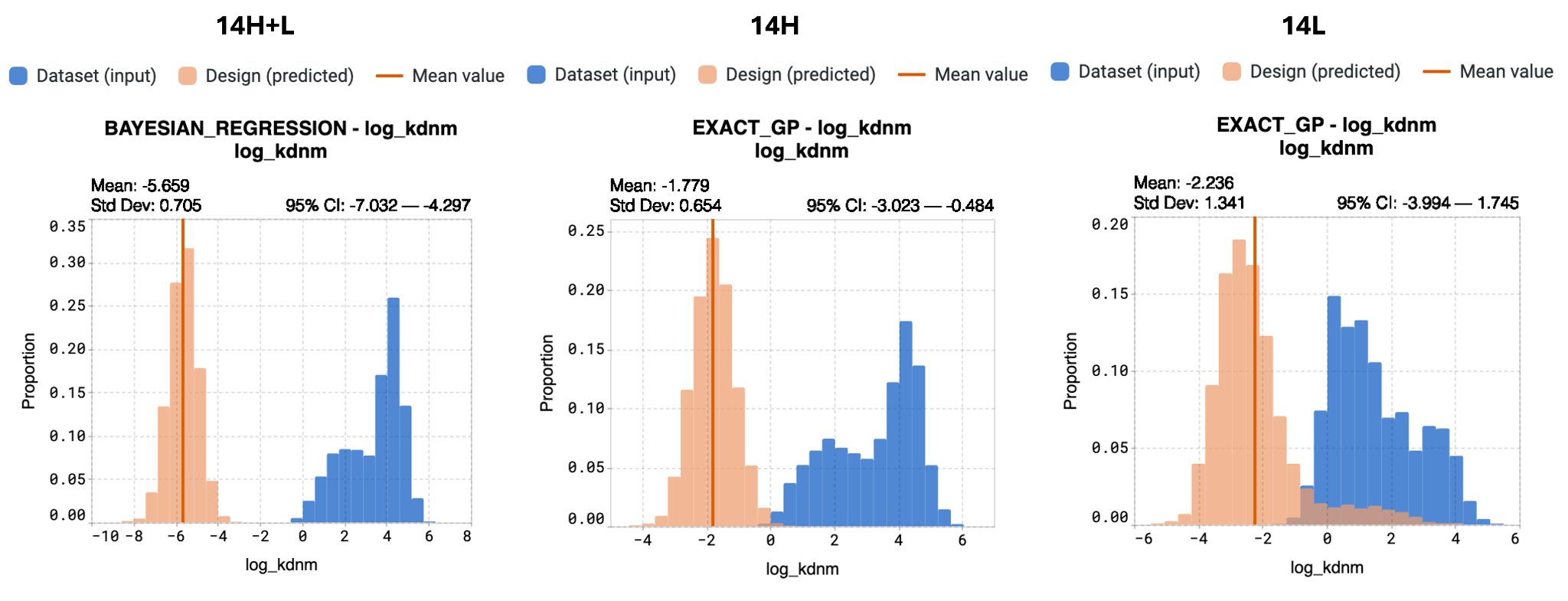
To train the custom model, we’ll navigate to an uploaded dataset and select Train Model. We’ll select the property “log_kdnm”, then select Start training to initiate the job. Once the job is submitted to the server, the OpenProtein.AI GPUs create a custom model specific to the targeted property. We’ll repeat this process for all three libraries. The figure below shows the 14H+L combined library.
Designing our variant library using the multichain data#
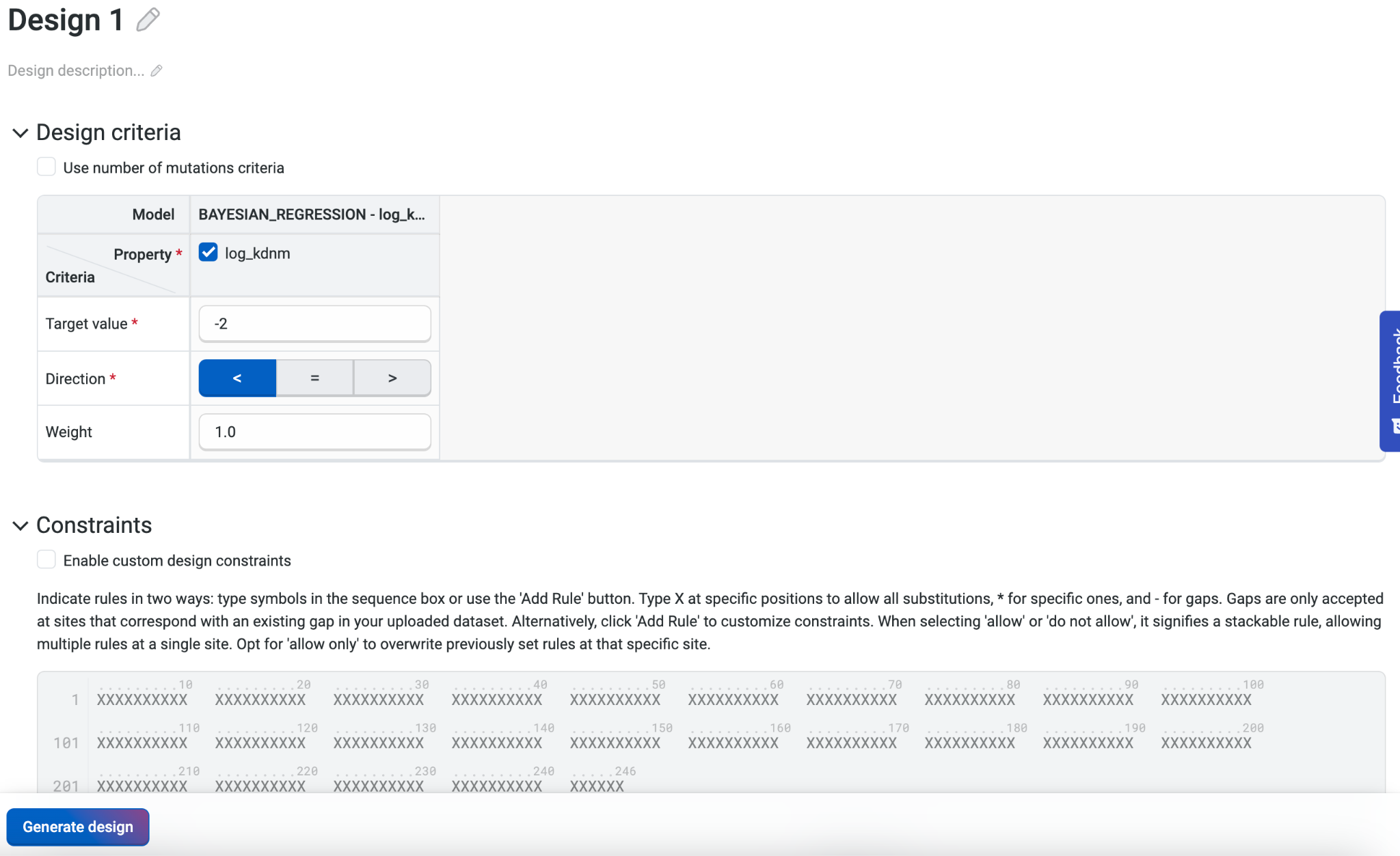
We are now ready to design a new variant library from the multichain dataset that we have uploaded (heavy+light chain).
From the Datasets component of our project, we’ll select Create Design. For this library, our goal is to design strong binders in the low picomolar affinity range. We will therefore specify a target affinity of less than 10pm, or -2 log_kdnm.
We recommend keeping the default setting for Number of design steps at 25 and Number of sequences per design step at 1024.
We’ll select Generate design to initiate our variant library design, which will be complete within a few hours.
Combining both the heavy and light chain at the same time as a single polypeptide allowed us to introduce mutations to both subunits in a single variant. This means we can explore a larger and more diverse design space, and also preserve any co-variations due to interchain interactions.
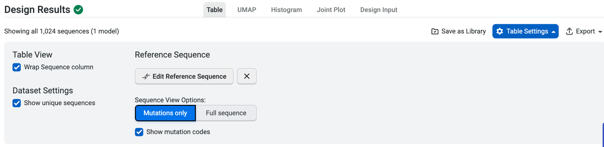
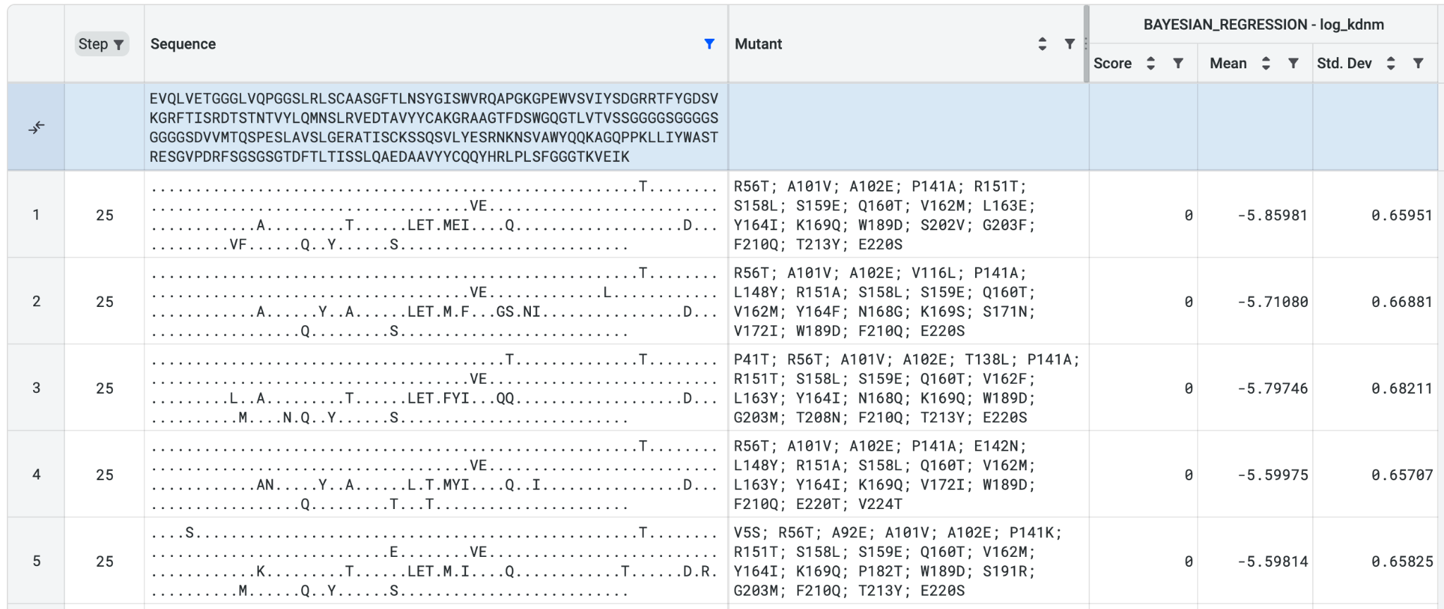
Once we have our design results, we can explore the introduced mutations. Our designed library contains a reference sequence, so we can select Table Settings and then check Mutations only to better visualize the mutations in the variants of the designed library.
We can see that there are mutations introduced to both the heavy and the light chain in a single variant. In the five variants below, R56T A101V A102E on the heavy chain are found with S158L S159E Q160T W189D on the light chain, suggesting possible interactions.
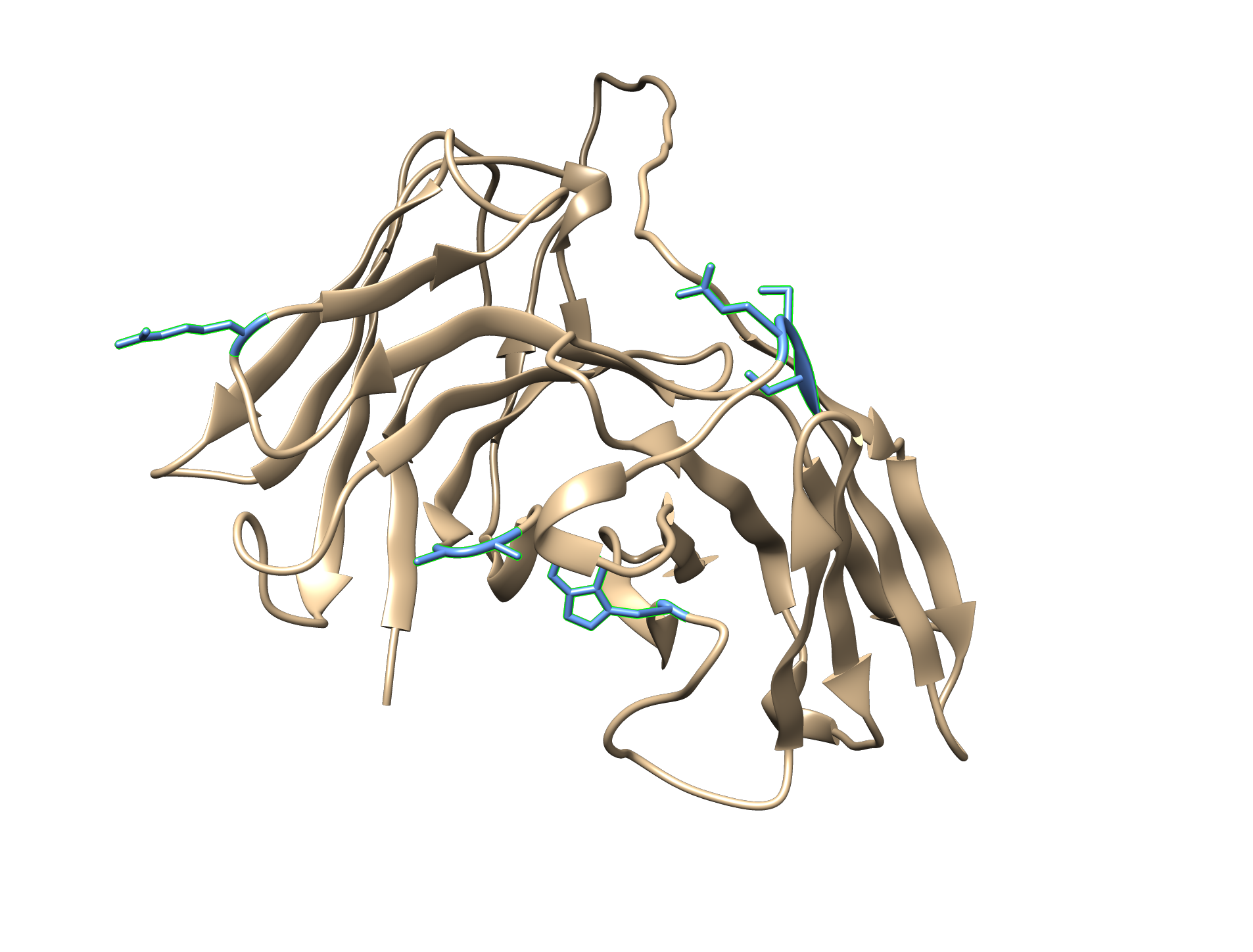
In the protein structure below, positions 101 and 102 lie close to position 189 (these positions are coloured cyan here), indicating that there may be interactions across both chains and the residues may co-vary together. Uncovering such potential interactions is only possible with multichain analysis.
We can repeat Design for the 14H and 14L standalone libraries, setting the similar target criteria of <-2.
Using different input libraries results in different library outputs with differing properties. We see that the designed library for the 14H+L multichain has much lower mean Kd. By simultaneously modifying both chains at the same time, we can achieve a better optimized design library.
Exporting the ML designed variant library#
We’ve successfully generated a new set of variants for 14H+L and are ready to move forward with getting data from our library.
First, we will need to save and export the sequences generated by OpenProtein.AI. We can save the results within our project, “Antibody optimization 14H+L”, by selecting Save as library, then adding a library name and description before selecting Save. We can also export all or some of the results as a CSV file by selecting Export. This file is ready to send to our gene synthesis company of choice.
Summary and next steps#
In this walkthrough, we demonstrated how to chain together multiple sequences in order to visualize a multimeric sequence using Structure Prediction. We also trained custom models to design an optimized library for the full multimeric protein. The subunits were mutated simultaneously, which highlighted key points of interaction.
Get started with OP Models here and Structure Prediction here.